NavList:


(Since I never know how the formatting will work out I am attaching a PDF also)

We have had some interesting discussions lately about improving the accuracy of our celestial
navigation. First we reexamined the old cocked hat and discovered that there are many new ways
to choose a center. We learned new words such as incenter, centroid, steiner point and
symmedian point. Then we moved on to trying to improve the accuracy of the individual LOPs
making up the cocked hat with some suggestions of averaging many sights, linear regression,
least squares, and the use of a predicted slope to identify �outliers� that should be eliminated
prior to averaging. My own opinion is that one sight each on two well spaced stars provides an
accurate enough fix for normal off shore navigation. Shoot a third star to eliminate certain types
of errors and you then have a fix that you can rely on in laying out the course for the next day.
But I can envisage some situations where it would make sense to try to improve the accuracy of
the fix such as when approaching land or when passing a mid-ocean reef. In these situations I
wouldn�t use the possibly more accurate fix to cut it closer to the danger but would use the
increased accuracy to provide more peace of mind.

Peter Fogg described a method of graphing the sights and comparing them with a line drawn on
the graph at the slope that the sights are expected to follow during the shooting period.. This
method had also been mentioned in Dutton�s. This is different than the other methods discussed
as this is to be the first step that could be used to identify data that should be eliminated prior to
applying the other techniques. I think that everyone will agree that clearly erroneous data should
be discarded but the question is how do you decide when data is so bad that it should be
eliminated. If you detect some obvious problem, such as realizing that your watch had stopped,
then the answer is easy. But when it is not so obvious then Fogg�s technique might make sense.
So how do we choose which points are far enough away from the expected sloped line to be
eliminated? I think a way to make this decision is to consider the normal Gaussian distribution. A
navigator should have a good idea, based on his experience, what his sigma should be. He might
have several, based on different observing conditions that he can apply in deciding which data
points should be rejected. If you take a thousand sights you should expect 50 to exceed 2 sigmas
and since this would be part of a normal distribution you should not exclude these points in
calculating an average. But if you only take five shots you should not expect any to exceed two
sigmas (though it is possible but highly unlikely) if they are part of a normal distribution. So my
take on this is that for a small number of shots you should exclude any that exceed two sigmas
since it is more likely that this is a result of some anomalous event and not part of a normal
distribution that should be included in the average.

I decided to try this with the data I had supplied for a series of sights of Venus taken on an
Atlantic crossing in 2009. Although I provided fifteen sights I will concentrate on only six as
they were taken in a six minute period while the others were taken over a much longer period of
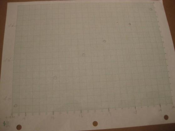
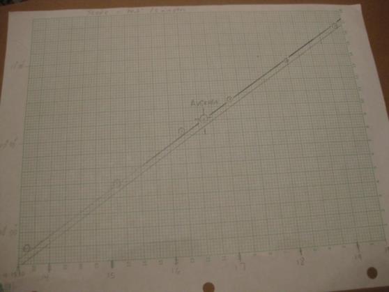
time. The first photo attached shows the six sights plotted on a graph, each grid line on the X axis
is one minute of altitude and the time intervals are three seconds. (The data for these shots is
attached at the bottom.) That was the easy part.

Now we have to decide how to draw the slope of the expected change in altitude in the six
minute period. There are two ways to compute this slope. You can pick an assumed position
nearby and calculate the computed altitude at the beginning and at the end (or near the end) of the
period, plot those two points and then draw a line between them. Off course a graph of computed
altitudes will not coincide with the plotted observed altitudes but the slope should be the same,
possibly being different my one tenth of a minute if there was a great enough change in the
altitudes to cause a slight change in the refraction corrections. If the ship was moving during the
shooting period then the slope will need to be adjusted to account for that also, either using a
second A.P. for calculating the second altitude or by using the H.O. 249 Motion Of the Observer
(MOO) table or the equivilent table that I computed and posted before.

http://fer3.com/arc/img/114591.moo-rev.pdf
http://www.fer3.com/arc/img/102321.moo%201.pdf

The other way is to determine the slope is by using the Motion Of the Body (MOB) correction
table in H.O. 249. This is easier and can be done without looking at the Almanac as the only
information needed is the DR latitude and the azimuth of the body, which can be measured
accurately enough for this purpose. You can also calculate this with the formula: Delta H = 15 x
cos latitude x sin azimuth, where Delta H = rate of change in arc minutes per minute of time.
To account for the movement of the vessel you can also use the MOO table from H.O. 249 or the
table I have previously posted that accomplishes the same thing.

http://www.fer3.com/arc/img/102321.mob%201.pdf

Using my data for this, my DR latitude was 14̊ 25' north and the azimuth of Venus was 103̊
true. We look at the H.O 249 MOB table (attached) and we find (by visual interpolation) the
altitude of the body is increasing 14.2' for every minute of time. For a five minute period this
would result in 71.0' increase in altitude. To allow for the movement of the ship, which was
sailing at 11 knots on a course of 251̊ true which placed Venus at a relative azimuth of 148̊, we
can look at the table I created for the Motion of the Observer for 11 knots and visually
interpolate between 140̊ and 160̊ relative azimuth and take out the correction of -0.8' for a five
minute correction. If you want to use the H.O. 249 MOO table (attached) take out the value for
550 knots and a relative azimuth of 148̊ which is -7.8' per minute of time. Divide by 100 to find
the correction for 5.5 knots which is - 0.078' and then multiply by two to find the correction for
11 knots resulting in -0.156' per minute. Multiply by 5 to find the total five minute Motion Of the
Observer correction which is -0.78' rounded to -0.8', the same as my table. Combining the
Motion Of the Observer and the Motion Of the Body correction and we find the slope to be 70.2'
for five minutes.

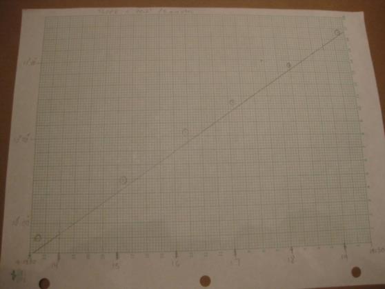
The second photo shows where I drew in the expected altitude slope. I just placed a dot at a
convienent point for the beginning of the line and then moved five minutes to the right and up
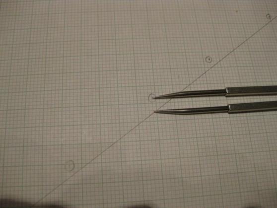
70.2', placed a dot and then drew a straight line between them. Then using a dividers (third
photo) I measured the distance of each point from the slope and got 3.8', 2.5', 4.1', 2.6', 1.9', and
1.1'. The average was 2.7' and I could move the sloped line up by this amount to draw the sloped
line through the sextant altitude points but this is not really necessary since we are looking to find
the displacement of the points from the average line. We can do this by simply subtracting 2.7'
from the already measured displacements resulting in residual displacements of 1.1', -0.2', 1.4',
-0.1', -0.8', and -1.6'.

I had found that the historical standard deviation of my sights is 1.433' so applying my two sigma
test to this data I find that none of the sights were displaced from the average slope line
exceeding 2.866', two sigmas, the largest being only -1.6'. Based on this rule I eliminated none of
the observations since there were no �outliers� in this data set. So using all the observation, I
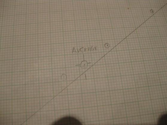
computed an average sextant altitude of 10̊ 35.7' and an average time of 9:16:36 Z. The third
photo shows this average point plotted. The forth photo shows the slope line moved up by 2.7' to
go through the data points.

The purpose for averaging and the other techniques is to improve the accuracy of the LOP. Since
I have gps positions for each of the sights, and for the average, we can see if averaging improved
the accuracy of the resulting LOP. The six intercepts are 0.7 T; 0.2 T; 1.3 T; 0.2 T; 0.5 A; and 0.8
A resulting in a standard deviation of 0.77 nm. The intercept for the average sight is only 0.1 T so
it appears that the averaging did improve the accuracy of the resulting LOP. Peter Hakel analysed
my data and, using his methodology, came up with an average observed altitude of 10̊ 27.7' at
9:16:54 Z. Computing an Hc for the gps coordinates at that time produces 10̊ 27.9' making the
intercept 0.2 A so his method also improved on the individual sights but not as well as the
simple average which was only 0.1 T.

Then there is the question of how many sights need to be averaged? Weems states that the error
in the average of a series of sights is determined by the square root of the number of sights. So to
halve the error you need to take 4 sights; to cut it to one-third requires 9 sights; one-fourth, 16
sights; one-fifth, 25; and one-tenth, 100 sights.

gl

------------------------------------------------------------------------------------------------------------------
Data:

Some of you have requested real data to use to experiment with various data massaging
techniques to improve the accuracy of observed altitudes. This data was obtained onboard the
Royal Clipper on a transatlantic crossing in 2009. I am providing the raw data for six
observations of Venus taken in a six minute period for you to number-crunch.

Greenwich date: November 6, 2009
All times are GMT with no watch error.
Height of eye: 33 feet.
Index error: + 1.3'.
Course: 251̊ true.
Speed: 11 knots.
Temp. 70 F
Pres. 1013 mb
Body: Venus.
Measured azimuth for the first shot was 102̊ true and for all the rest was 103̊ true.

Approximate location at middle of series was 14̊ 25' north, 55̊ 00' west.

I have the GPS coordinates for each shot and will supply them later so we can see how well the
number-crunching did.

Number Time Sextant altitude GPS

1 9:13:38 9̊ 54.8' 14̊ 25.9' N, 54̊ 59.7'W

2 9:15:06 10̊ 14.6' 14̊ 25.8' N, 55̊ 00.0'W

3 9:16:13 10̊ 31.2' 14̊ 25.7' N, 55̊ 00.2'W

4 9:17:06 10̊ 42.6' 14̊ 25.7' N, 55̊ 00.3'W

5 9:18:15 10̊ 57.9' 14̊ 25.6' N, 55̊ 00.5'W

6 9:19:22 11̊ 13.1' 14̊ 25.5' N, 55̊ 00.7'W

-----------------------------------------------------------------------------------------------------------------

My average 9:18:36 10̊ 35.7' 14̊ 25.7' N, 55̊ 00.2'W

-----------------------------------------------------------------------------------------------------------------
Hakel�s Ho 9:16:54 10̊ 27.7 14̊ 25.7' N, 55̊ 00.3'W

I have another 6 shots of Venus taken a little bit earlier the same day but over a period of 21
minutes which you may want to combine with the other six shots, or not, due to the long time
span. I have 3 more shots of Venus taken slightly later that you can also combine, or not, due to
the long time period. In total, there are 15 shots taken over a 39 minute period. All the rest of the
conditions remain the same except for the measured azimuths for the earlier shots.

Earlier series.

The measured azimuth to the first two shots was 101̊ true and for the last four shots the azimuth
was 102̊ true.

Number Time Sextant altitude GPS

A1 8:49:09 4̊ 14.8' 14̊ 27.4' N, 54̊ 55.4'W

A2 8:51:04 4̊ 44.1' 14̊ 27.3' N, 54̊ 55.7'W

A3 9:06:52 8̊ 20.6' 14̊ 26.3' N, 54̊ 58.5'W

A4 9:08:18 8̊ 40.3' 14̊ 26.2' N, 54̊ 58.8'W

A5 9:09:28 8̊ 55.9' 14̊ 26.2' N, 54̊ 59.0'W

A6 9:10:32 9̊ 10.5' 14̊ 26.6' N, 54̊ 59.2'W

.

The third series, all the measured azimuths were 103̊ true.

B1 9:22:53 12̊ 01.8' 14̊ 25.3' N, 55̊ 01.3'W

B2 9:24:06 12̊ 19.1' 14̊ 25.3' N, 55̊ 01.6'W

B3 9:27:43 13̊ 09.5' 14̊ 25.1' N, 55̊ 02.2'W

----------------------------------------------------------------
NavList message boards and member settings: www.fer3.com/NavList
Members may optionally receive posts by email.
To cancel email delivery, send a message to NoMail[at]fer3.com
----------------------------------------------------------------